Blog

Learning action-angle coordinates with a Koopman-inspired symplectic autoencoder

I have been working on a neural-network approach to learning action-angle coordinates directly from orbital trajectories, while also recovering orbital frequencies and a Hamiltonian-like energy map. The longer-term goal is to make action-angle calculations more flexible in realistic Galactic potentials, but for now I only want to show the one-dimensional validation tests publicly.

So this post is intentionally narrow: a brief bit of context, the core idea, and the 1D results in the harmonic oscillator and isothermal slab. The broader axisymmetric results are being held back for now because that work is intended for publication.

PyTorch Hamiltonian Dynamics Koopman Neural Networks Action-Angle Coordinates Galactic Dynamics

Note. This is a public snapshot of the project. I am only showing the one-dimensional tests here; the more extensive higher-dimensional results are deliberately omitted while the work is being prepared for publication.

Why action-angle coordinates matter

Action-angle coordinates are one of the most natural languages for regular Hamiltonian motion. In integrable systems, the actions are constants of motion, while the angles evolve linearly in time. That makes them extremely useful both for equilibrium modelling and for studying disequilibrium structure in the Milky Way.

In Galactic dynamics, these coordinates are especially valuable because distribution functions are often written in terms of the actions, and because action-angle structure can reveal moving groups, resonances, phase mixing, spiral features, and bar-driven dynamics much more cleanly than ordinary phase-space coordinates alone. The difficulty is that action-angle coordinates are only known analytically in a few ideal potentials.

This project asks whether a useful action-angle representation can be learned directly from trajectories while still respecting Hamiltonian structure.

The idea in one paragraph

The model is a symplectic autoencoder. It learns an invertible map from phase-space coordinates into a latent space where each degree of freedom is represented by a two-dimensional plane. In that latent space, the dynamics are constrained to look like simple rotations, so the radius of each latent pair behaves like an action and the phase behaves like an angle.

A separate small neural network then learns the frequency map and another learns a scalar energy-like function, with the model encouraged to satisfy the Hamiltonian relation dH/dJ ~ Omega(J). The point is not just to reconstruct trajectories, but to make the latent variables physically interpretable.

A short mathematical sketch

The autoencoder learns an encoder Psi and decoder Phi so that phase-space evolution is approximately conjugate to a simpler latent evolution,

x_k+1 ≈ Φ(K(Ψ(x_k)))

Each latent pair is interpreted as a complex coordinate whose radius encodes an action and whose phase encodes an angle,

ψ_j = u_j + i v_j = √(2J_j) exp(iθ_j)

The latent step is then just a rotation,

[u_j, v_j]_k+1^pred = R(φ_j) [u_j, v_j]_k, with φ_j = ω_jΔt

That rotation preserves radius exactly. So the latent action is conserved by construction, while the frequency map is learned from data.

Model construction

I am skipping most of the training details here, but the architecture matters. The encoder is built from symplectic coupling layers, so the learned map is invertible and structure-preserving by construction. The decoder is simply the inverse map. That helps separate two different questions: whether the representation itself is good, and whether the learned latent evolution is good.

In one dimension, the model is relatively small: an 8-layer symplectic encoder/decoder, plus compact MLPs for the frequency map and the Hamiltonian regressor. The two validation problems are a harmonic oscillator, where the action-angle structure is analytically known, and an isothermal slab, where the frequency varies non-trivially with action.

1D tests

The first set of checks is deliberately simple. If the model cannot recover stable actions, angles, and frequencies in one dimension, there is no point pretending it will behave sensibly in more realistic Galactic potentials.

Harmonic oscillator

Potential: Phi(z) = omega_0^2 z^2 / 2 with omega_0 = 0.5. Here the true frequency is constant, so this is the cleanest sanity check.

Isothermal slab

Potential: Phi(z) = 2 sigma^2 log(cosh(z / 2 z_0)) with sigma = 1 and z_0 = 1. This is more interesting because the oscillation frequency decreases with action.

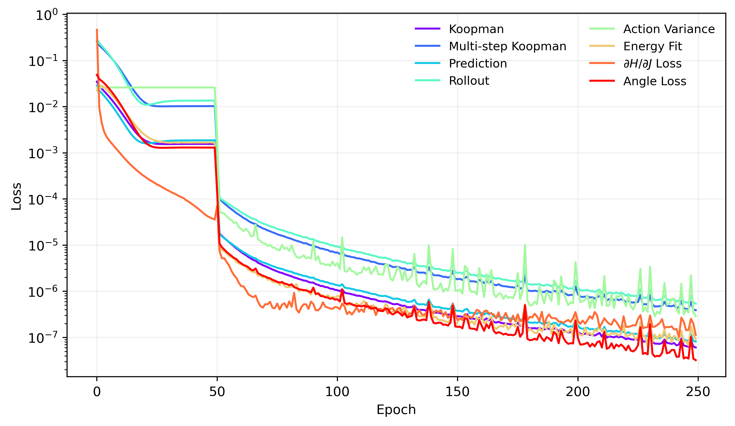
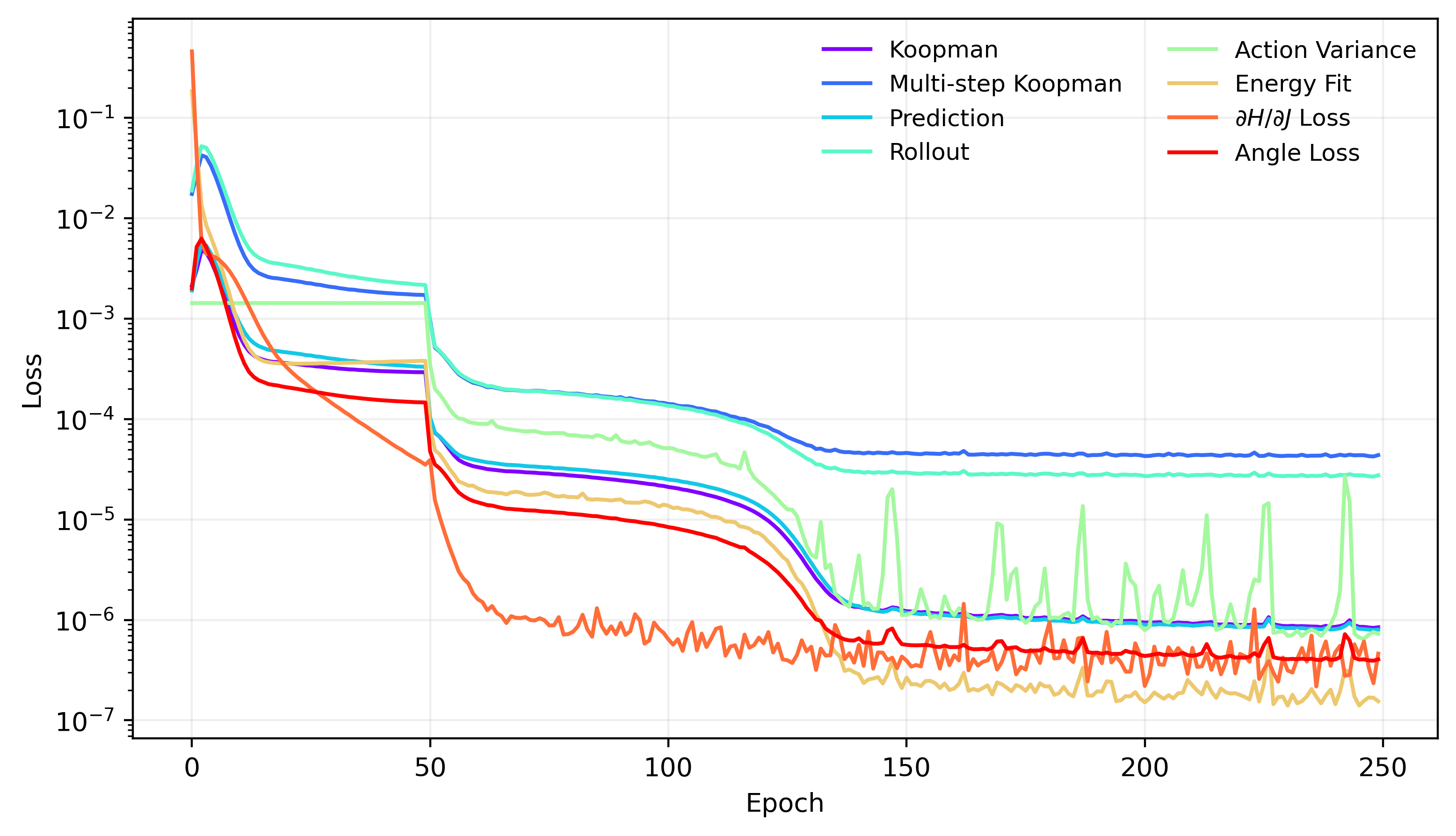
Training curves

Both 1D experiments train cleanly. I am not showing every individual loss term here, but the main point is that the one-step, rollout, and physics-informed objectives settle to small values by the end of training in both systems.

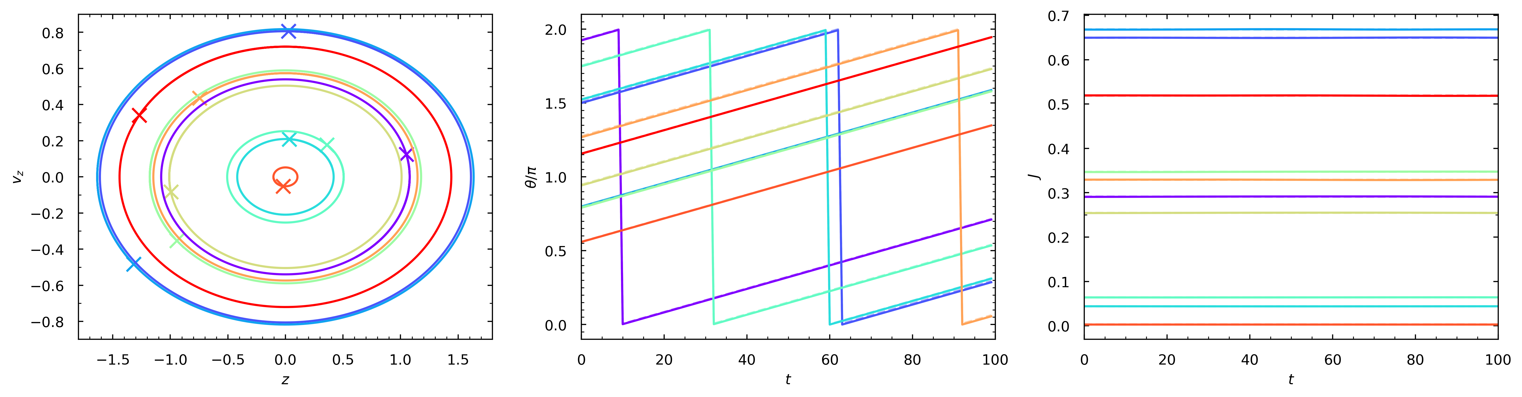
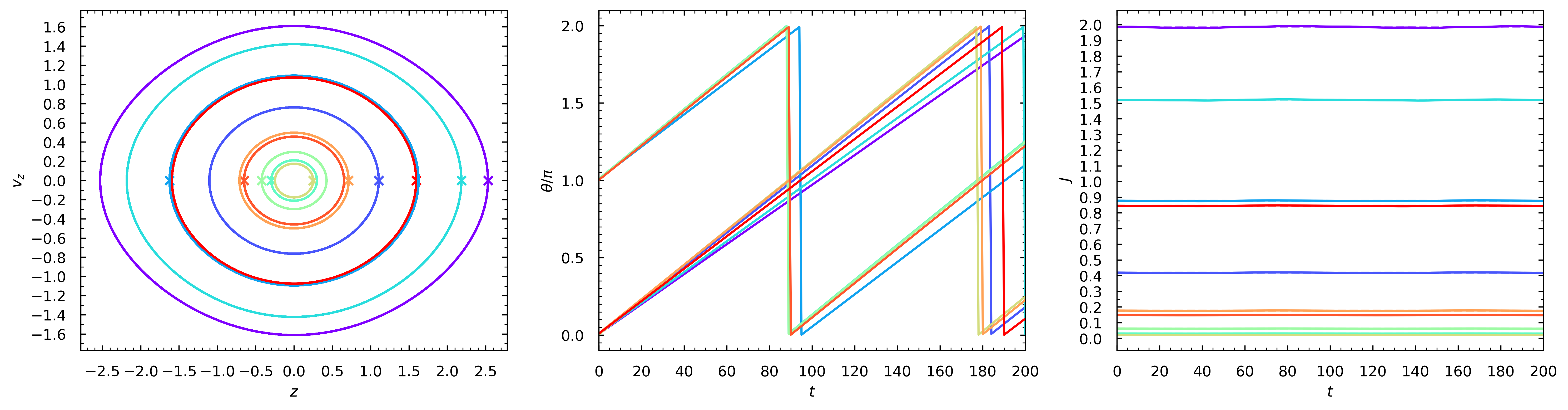
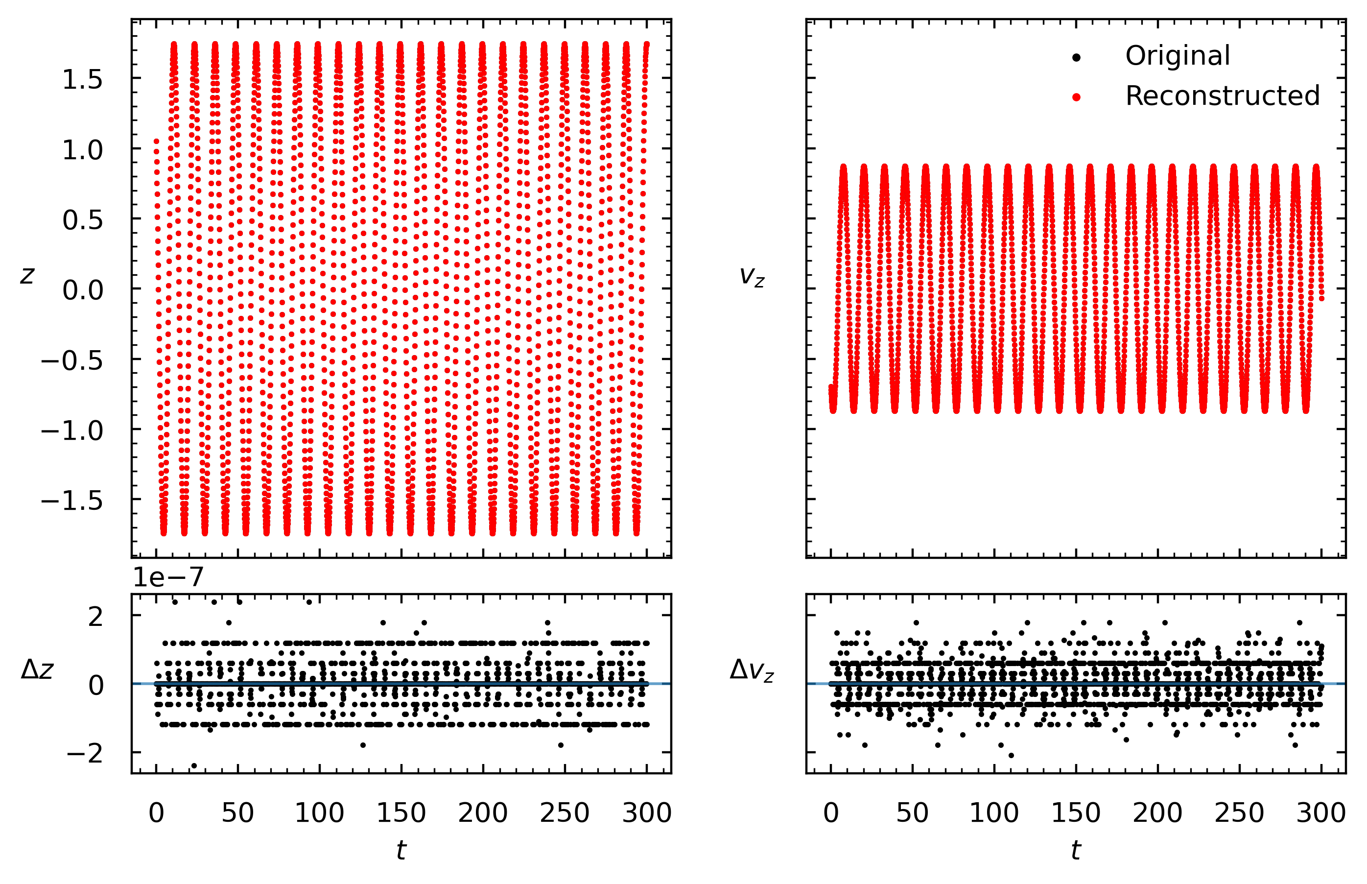
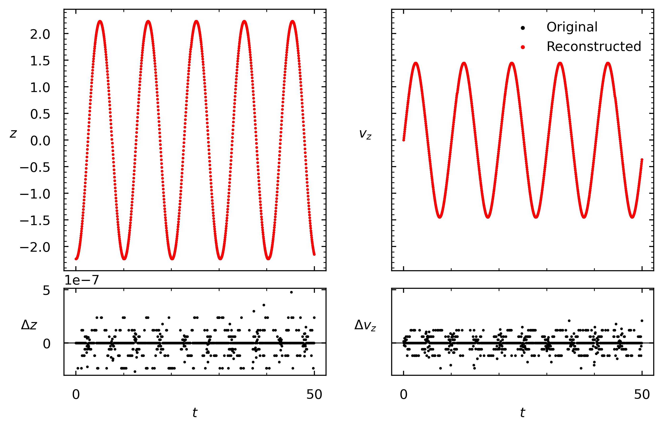
Training loss curves for the harmonic oscillator model — **Harmonic oscillator.** Training losses decrease smoothly and remain well controlled throughout optimisation.

Training loss curves for the isothermal slab model — **Isothermal slab.** The same architecture also converges cleanly when the frequency depends on action.

Recovered actions and angles

The most important qualitative check is whether the learned action stays nearly constant along each orbit, while the learned angle tracks a linearly advancing variable. That is exactly what the model recovers in both 1D examples.

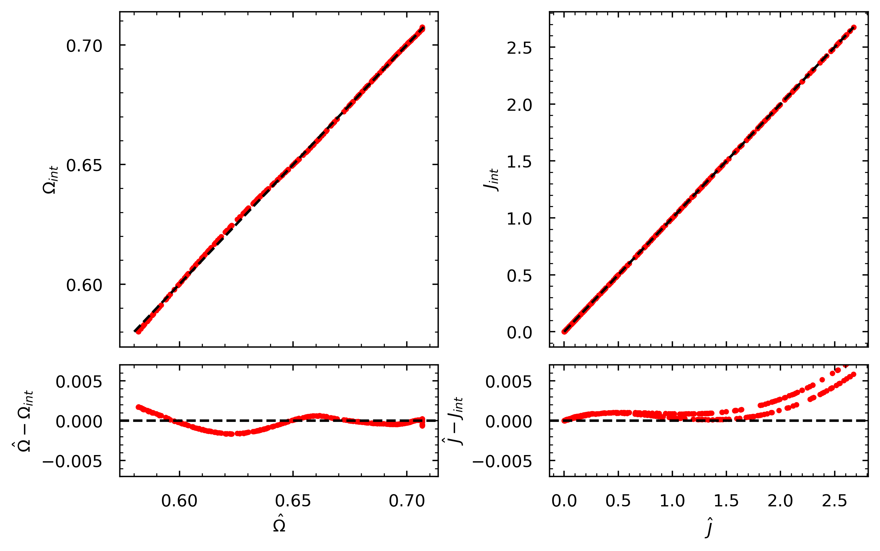
Harmonic oscillator phase space with learned actions and angles — **Harmonic oscillator.** The learned angle closely tracks the analytic angle, and the learned action remains effectively constant along the trajectory. In this 1D test, the mean-square errors are approximately 10^-9 for the frequency and 10^-7 for the action.

Isothermal slab phase space with learned actions and angles — **Isothermal slab.** The same latent construction remains useful in a system where the frequency is not constant across orbits.

Frequency-action comparison in the isothermal slab

For the isothermal slab, I compared the learned actions and frequencies against numerical reference values obtained from the standard orbit integrals,

J_z = (1 / 2π) ∮ v_z dz, Ω_z(J) = 2π (∮ dz / v_z)^-1

The agreement is good: the absolute residuals stay within about 0.005, which is more than enough to show that the model is learning a sensible action-frequency relationship rather than just memorising trajectories.

Comparison of learned and numerically integrated actions and frequencies in the isothermal slab — **Isothermal slab validation.** Learned actions and frequencies agree well with numerically integrated reference values, with absolute residuals within roughly 0.005.

Reconstruction and inverse mapping

Another useful check is to separate reconstruction quality from dynamical prediction. If a state is encoded and immediately decoded, the reconstruction is essentially exact up to numerical precision. That confirms that prediction errors are driven by the learned latent evolution and frequency map, not by a failure of invertibility in the symplectic encoder-decoder pair.

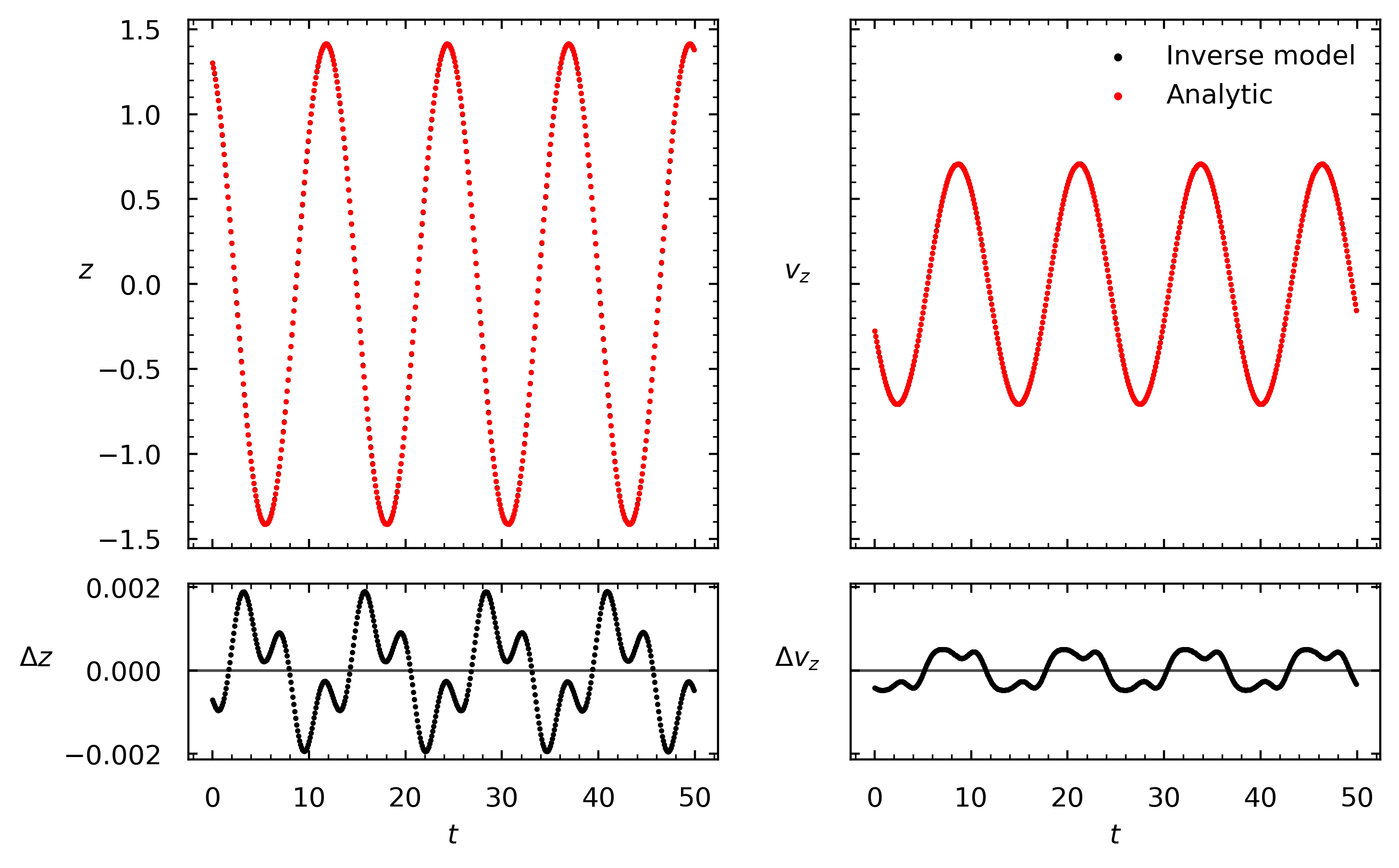
In the harmonic oscillator, the learned inverse map can also be used to generate an orbit directly from an initial action-angle point. The decoded trajectory stays close to the analytic solution, with residuals at the 10^-3 level and no obvious secular drift over multiple periods.

Harmonic oscillator reconstruction from encode-decode — **Harmonic oscillator reconstruction.** Encoding and decoding the same states gives reconstruction residuals close to numerical precision.

Isothermal slab reconstruction from encode-decode — **Isothermal slab reconstruction.** The invertible symplectic map remains stable away from the analytic toy case.

Harmonic oscillator rollout generated from learned inverse map — **Inverse rollout in the harmonic oscillator.** Starting from an initial action-angle point, the model generates a stable decoded orbit that remains close to the analytic trajectory, with residuals typically around 10^-3.

What I think is actually interesting here

There is no shortage of machine-learning models that can fit trajectories. The more interesting question is whether a model can discover coordinates that behave like the right physical variables. These 1D tests suggest that a symplectic autoencoder plus constrained latent rotations is a plausible route to doing exactly that.

The real challenge is of course the higher-dimensional Galactic case, where actions and frequencies are more subtle and the benchmark is much harsher. I am deliberately not showing those results yet, but the 1D experiments are the reason I think the larger programme is worth pursuing.

References

Antoja et al. (2023). Vertical waves, ridges and phase-space spirals in the Milky Way. ADS

Binney (2010). Distribution functions for the Milky Way. ADS

Bramburger (2024). Introduction to Koopman Operator Theory and Its Applications.

Brunton, Budišić, Kaiser, and Kutz (2022). Modern Koopman Theory for Dynamical Systems. arXiv

Greydanus, Dzamba, and Yosinski (2019). Hamiltonian Neural Networks. arXiv

Gaia Collaboration (2023). Gaia Data Release 3. ADS

Hunt et al. (2019). Kinematic substructure in action space with Gaia. ADS

Ibata et al. (2021). ACTIONFINDER: deep learning of canonical transformations. ADS

Jin et al. (2020). SympNets: intrinsic structure-preserving neural networks for Hamiltonian systems. arXiv

Koopman (1931). Hamiltonian systems and transformation in Hilbert space.

Lusch, Kutz, and Brunton (2018). Deep learning for universal linear embeddings of nonlinear dynamics. Nature Communications

Palicio et al. (2023). Tracing spiral arms in action space.

Paszke et al. (2019). PyTorch: An Imperative Style, High-Performance Deep Learning Library. arXiv

Piffl et al. (2014). Constraining the Galaxy's mass distribution with realistic action calculations. ADS

Sanders and Binney (2016). Methods for computing actions, angles and frequencies in Galactic potentials. ADS

Williams, Kevrekidis, and Rowley (2015). A data-driven approximation of the Koopman operator: extending dynamic mode decomposition. Journal of Nonlinear Science